All The Language

This post is a continuation of Constraint Grammar can count!, in which I talked a bunch about how expressive constraint grammar is. Now, for most of that post, what I actually meant was the fragment of constraint grammar where you only use the REMOVE rule.¹ However, I always had the suspicion that I’d be pretty easy to simulate a Turing machine using only the ADDCOHORT and REMCOHORT commands, treating the list of cohorts as the Turing machine’s tape—and I don’t think I was the only one to feel that way.

Now, this would be wonderful news. It would prove that ADDCOHORT and REMCOHORT are Turing-complete—given that VISL CG-3 itself is a pretty decent proof that we can run constraint grammars on a universal computer. Not only that, but VISL CG-3 is an extremely optimized piece of software—so the fact that we could compile any Turing machine to VISL CG-3 would be great news for the HPC community².

With all this in mind, I decided to finally work out the details of this compiler I had had tumbling around in my brain for the past months. Turns out, it’s kinda nice.

For this post, we’ll encode the first Turing machine program I could find, using a quick search, as a constraint grammar, using only ADDCOHORT and REMCOHORT³ I’ll try to explain the general principle as we go. But first, I should probably briefly go over how a Turing machine works—though I hope you’ll forgive me if I’ll be a little informal. Heads-up: If you don’t want to read through a whole bunch about Turing machines, it’s probably best to skip right to the meat.

So what’s this Turing machine business?

A Turing machine is a tiny machine, which sits whirring away on top of an infinite roll of tape. It has a head, which hoovers over the tape, and reads and writes whatever cell it happens to hoover over. It also has a state. This is basically saying that it can remember what it was doing, but practically speaking this’ll be some number. The number of the thing it was supposed to be doing. It was never supposed to be built, but of course someone did:

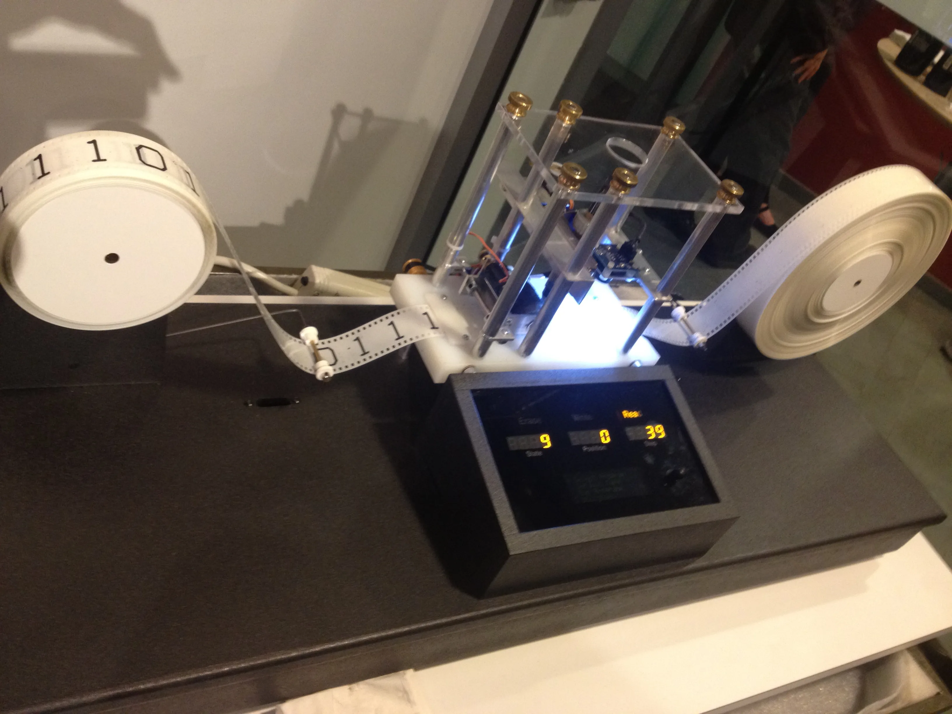
Actually, many people have built one. Out of everything from wood and scrap metal, to Legos, to artificial muscle.

Anyway. What makes every Turing machine special is that each has it’s own unique table, which contains its own unique program. At every step, the Turing machine will use its head to read the cell it’s hoovering over, and then sorta feel its state, and it will consult the great big (or sometimes small) table of its program. The table will then tell it what to do. What it should write over the thing it just read, what its next state should be, and whether it should whirr the tape to the left or to the right. It’ll do this until the table says it should enter its stop state. Then it stops. Some Turing machines have faulty tables, which never let it reach a stopping state.

Now, it just so happens that the first search result for “Turing machine example program” on the day I wrote this post was a machine which increments binary numbers, and its table looked like this:

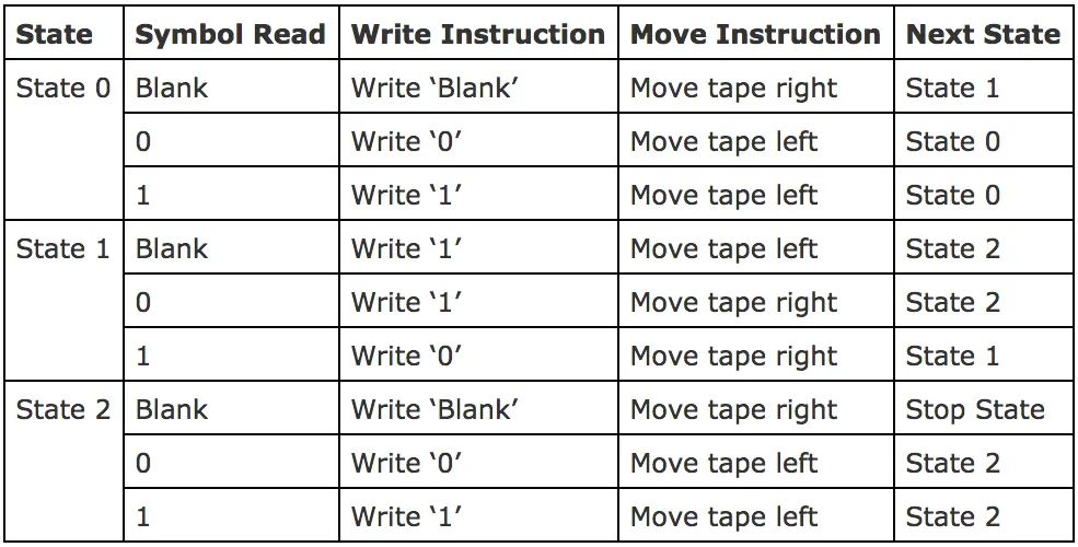
These programs are a little hard to read, so let’s go over what the Turing machine will be doing at each of these states.

State 0 The machine expects its input—that number we’re going to increment—to already be written on the tape. However, it doesn’t trust us to place its head directly at the beginning of said number. So, state 0 is there so that wherever in the number we put its head, it will move right to the start. Then it continues in state 1.

State 1 All the real work is done in state 1. In state 1, the Turing machine is in the business of progressivly moving its head to the right. It will overwrite any 1 it meets with a 0. But if it ever reads a 0 or a blank, it will write a 1 and continue in state 2.

State 2 A brief check with your binary arithmetic will tell you we’ve already incremented the number in the previous state. So what is state 2 there for? It does the same thing as state 0. For reasons of cleanliness, and being a good bot, it moves its head back to the beginning of the number. And when it has done that, it stops.

Below is the trace for the machine incrementing the number 11 to 12, or 1011 to 1100 in binary. I’ve put a 🤖, to show you where the machine is looking:

_	_ 🤖	1	1	0	1 # 0: Read 1, Write 1, Move ←
_ 🤖	_	1	1	0	1 # 0: Read _, Write _, Move →
_	_ 🤖	1	1	0	1 # 1: Read 1, Write 0, Move →
_	_	0 🤖	1	0	1 # 1: Read 1, Write 0, Move →
_	_	0	0 🤖	0	1 # 1: Read 0, Write 1, Move ←
_	_	0 🤖	0	1	1 # 2: Read 0, Write 0, Move ←
_	_ 🤖	0	0	1	1 # 2: Read 0, Write 0, Move ←
_ 🤖	_	0	0	1	1 # 2: Read _, Write _, Move →
_	_ 🤖	0	0	1	1 # Stop

Great! So now we’ve got that out of the way, let’s have a look at implementing this machine in VISL CG-3, because why not?

VISL CG-3 Turing Machines

We’re going to represent the Turing machine’s tape as a list of cohorts. This means that when we pass in the number 11, we pass VISL CG-3 the following text:

"<Cell>" "1"
"<Cell>" "1"
"<Cell>" "0"
"<Cell>" "1"

We will take a cue from the nice infix notation we used above, and write the current state to the tape, right before the cell which the head is currently on. For instance, the third row in the execution trace above would be written as:

"<Cell>" "0"
"<State>" "State1"
"<Cell>" "1"
"<Cell>" "0"
"<Cell>" "1"

To start off, our constraint grammar will add a cohort for the start state. It’ll add it right before the first cell of our input. This kind-of makes the whole of state 0 superfluous, but we’ll keep it anyway, for good form:

BEFORE-SECTIONS
ADDCOHORT ("<State>" "State0") BEFORE ("<Cell>") IF (-1 (>>>));

Now the meat. We will encode the program of our Turing machine. This is a recursive specification, we we’ll need to wrap it in a SECTION. First, we mark the current state cohort and the cell we’re reading as old:

ADD ("<State>" "OLD") ("<State>");
ADD ("<Cell>" "OLD") ("<Cell>") IF (-1 ("<State>" "OLD"));

I realise that these are ADD commands, and I promised to only use ADDCOHORT and REMCOHORT, but hear me out. We can simulate this usage of ADD by adding a cohort "<Old>" after the cohort we’re marking. However, every time we now select a cohort using e.g. ("<Cell>" "OLD"), we’d have to change this to (0 ("<Cell>") LINK 1 ("<Old>"))… and we’d have to take into account the expected number of "<Old>" cohorts, and move every selection by that. Anyway, it wouldn’t be pretty. So please allow me this one thing. Ok?

Back to our scheduled program. Once we’ve marked our old state cohort and the cell we’re reading as old, we can introduce new ones. We will compile every single entry in the Turing machine’s program to two rules. One which introduces the next state, and one which writes a new cell to replace the old one. For instance, the rule which says that “if we are in state 1, and we read a 1, then we write a 0, move the tape to the right, and continue in state 1,” is compiled to the following two rules:

ADDCOHORT ("<State>" "State1")
   BEFORE ("<Cell>")
       IF (-2 ("<State>" "State1" "OLD") LINK
            1 ("<Cell>" "1" "OLD"));
ADDCOHORT ("<Cell>" "0")
    AFTER ("<Cell>" "1" "OLD")
       IF (-1 ("<State>" "State1" "OLD"));

And the rule which says that “if we are in state 1, and we read a blank, then we write a 1, move the tape to the left, and change to state 2” is compiled to the following two rules:

ADDCOHORT ("<State>" "State2")
   BEFORE ("<Cell>")
       IF (1 ("<State>" "State1" "OLD") LINK
           1 ("<Cell>" "_" "OLD"));
ADDCOHORT ("<Cell>" "1")
    AFTER ("<Cell>" "_" "OLD")
       IF (-1 ("<State>" "State1" "OLD"));

In both pairs, the first rule inserts the next state in the appropriate place, and the second rule inserts the newly written cell after the one marked as old.

After all these rules—of which at most one pair will match, because we check for both the state and the cell marked as old—we clean up, simply removing every cohort marked as old:

REMCOHORT ("<State>" "OLD");
REMCOHORT ("<Cell>" "OLD");

This cycle of marking as old, applying the transitions, and removing the old cohorts will repeat until there are no further changes. Since there are no transitions which match on a stop state, the repetitions will stop here, and the stop state will be marked as old and removed.

Finally, because moving the head back to the start of the number is rather pointless in this implementation, we have a final cleanup step. We remove any leading or trailing blank cells:

AFTER-SECTIONS
REMCOHORT ("<Cell>" "_") IF (NOT -1* SYMB);
REMCOHORT ("<Cell>" "_") IF (NOT  1* SYMB);

Hooray! We’ve implemented a Turing machine! Or have we? There’s one tiny issue with the above implementation. Our little Turing machine sits whirring on top of an infinite amount of tape. Here, our implementation only ever writes to cells which were already filled in the input. This means we’ve actually been implementing a linear bounded automaton all this time—i.e. we’ve proven that ADDCOHORT and REMCOHORT cover at least the context-sensitive languages! But really, we’d like to be able to simulate Turing machines, so…

There is a simple way to extend this framework to Turing machines. We add two rules, right at the start of the SECTION, which simply add more blank cells to the edges of the tape whenever the head gets too close:

ADDCOHORT ("<Cell>" "_")
   BEFORE ("<State>")
       IF (-1 (>>>));
ADDCOHORT ("<Cell>" "_")
    AFTER ("<Cell>")
       IF (0 (<<<) LINK -1 ("<State>"));

The first of these rules adds a blank cell at the beginning if the state cohort is the first cohort. The second adds a blank cell at the end if the state cohort is the second-to-last cohort—because, remember, we are reading the cell right after the cohort.

Now if you’re thinking “VISL CG-3 is known for being fast; I can’t wait to compile all my code to it!” then I have to tell you—way ahead of you. I’ve implemented this TM to CG compile as a small Haskell library, in addition to a small Turing machine interpreter, so you can really see just how much time you’re saving. I’ve also implemented my example machine, the binary successor function, and wrote a set of QuickCheck functions which compare:

• Haskell’s (+1);
• the interpreted binary successor machine; and
• the compiled binary successor in VISL CG-3.

Turns out, everthing works!⁴ If you want to have a go—maybe implement that sorting algorithm so you can really do a speed comparison—the library is available on my Github, and you can get VISL CG-3 on the internet.